Modifying Solenoids

Solenoids can be modified to change the density of the DNA. Here we explore how this works.

The call to the Solenoid function is as follows:

dna.Solenoid(
    voxelheight: float = 750,
    radius: float = 100,
    nhistones: int = 38,
    histone_angle: float = 50,
    twist: bool = False,
    chain: int = 0,
)

These numbers are a realistic model for how much Solenoidal DNA packs.

Unchanged, this will build a solenoid - 750 nm tall - histones centered 100A from the central axis - 38 histones - histones tilted at 50°.

Histones are always placed 60° apart going around the circle

It is recommended that you run this example inside a Jupyter environment rather than a VSCode or similar environment

This requires the mayavi jupyter extension jupyter nbextension install --py mayavi --user

import sys
from pathlib import Path

try:
    from fractaldna.dna_models import dnachain as dna
except (ImportError, ModuleNotFoundError):
    sys.path.append(str(Path.cwd().parent.parent.parent))
    from fractaldna.dna_models import dnachain as dna

import matplotlib.pyplot as plt
from mayavi import mlab

# Disable this option for interactive rendering
mlab.options.offscreen = True

# Enable this option for an interactive notebook
# mlab.init_notebook()

Varying Voxel Height

Varying the voxel height will compact and extend the DNA.

chain_750 = dna.Solenoid(voxelheight=750)
# MayaVI plots are best for visualisation here
plot = chain_750.to_line_plot()

# Save the figure
plot.scene.save_jpg("single_solenoid_750A.jpg")

# In an interactive notebook, you can refer to the figure to
# interact with it.
plot

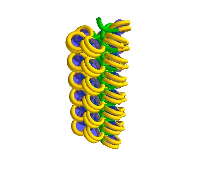
750 Å section, 38 histones

# Make a straight solenoid in a 500 Å box
chain_500 = dna.Solenoid(voxelheight=500)
# MayaVI plots are best for visualisation here
plot = chain_500.to_line_plot()

# Save the figure
plot.scene.save_jpg("single_solenoid_500A.jpg")

# In an interactive notebook, you can refer to the figure to
# interact with it.
plot

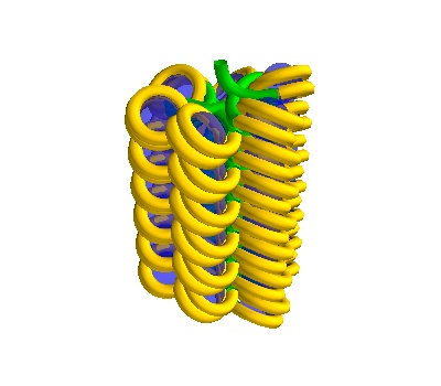
500 Å section, 38 histones - the DNA is more compacted (and the DNA could have overlaps).

Changing the number of Histones

When making DNA shorter (or longer), you should change the number of histones appropriately.

In general, you’ll want to keep the linear density of histones roughly constant (around 51/1000Å)

# Make a turned solenoid in a 750 Å box
chain = dna.Solenoid(voxelheight=500, nhistones=25)
# MayaVI plots are best for visualisation here
plot = chain.to_line_plot()
plot.scene.save_jpg("single_solenoid_500A_25histones.jpg")

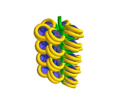
A 500Å long solenoid

If you need to make DNA a little denser, try increasing the linear density of DNA

# Make a turned solenoid in a 750 Å box
chain = dna.Solenoid(voxelheight=750, nhistones=42)
# MayaVI plots are best for visualisation here
plot = chain.to_line_plot()
plot.scene.save_jpg("single_solenoid_750A_42histones.jpg")

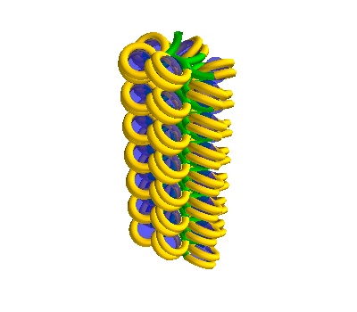
750Å strand, 42 histones

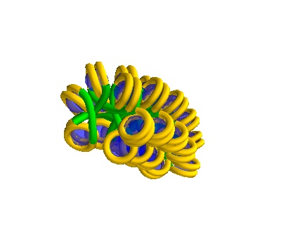
Turned Solenoids follow the same principles

They are actually based on the spacing that a straight solenoid would have, so the voxelheight and nhistones correspond to their straightened equivalents, and the linear density of histones is what is conserved.

The radius of curvature is half the voxel height.

Be particularly careful to ensure there are no overlapping molecules on the internal curve.

chain = dna.TurnedSolenoid(voxelheight=750, nhistones=42)
# MayaVI plots are best for visualisation here
plot = chain.to_line_plot()
plot.scene.save_jpg("turned_solenoid_750A_42histones.jpg")

750Å strand, 42 histones

It is important to inspect the result to make sure there aren’t placements where you don’t expect

With a voxelheight of 750Å, we expect bounds in the range

-375 < X < 375 -375 < Y < 375 0 < Z < 750

chain_df = chain.to_frame()

chain_df["max_extent"] = chain_df[["size_x", "size_y", "size_z"]].max(axis=1)

# What are the bounds of the box?
print(
    "X Bounds:",
    (chain_df["pos_x"] - chain_df["max_extent"]).min(),
    (chain_df["pos_x"] - chain_df["max_extent"]).max(),
)
print(
    "Y Bounds:",
    (chain_df["pos_y"] - chain_df["max_extent"]).min(),
    (chain_df["pos_y"] - chain_df["max_extent"]).max(),
)
print(
    "Z Bounds:",
    (chain_df["pos_z"] - chain_df["max_extent"]).min(),
    (chain_df["pos_z"] - chain_df["max_extent"]).max(),
)

Example Output

X Bounds: -130.5016837010315 371.3927605800866
Y Bounds: -152.83468961083372 148.26998187713423
Z Bounds: 0.04677445755690002 483.71674638609016

Exporting Solenoidal DNA to CSV

# This too can be exported to a dataframe of basepairs

# let's shift in so that it starts at z=-750/2, not at z=0
chain.translate([0, 0, -750.0 / 2.0])

# and then make it into a data frame
chain.to_frame()

# And a second data frame of histones
# This can be joined to the base pairs frame, assuming a sufficient handling of
# the missing strand index, and the relation between the base pair and histone index.
chain.histones_to_frame()